Deriving CQL-SAC | vernonwu

Readers are recommended to have prior knowledge for Reinforcement Learning basics. A good tutorial can be found here.

Introduction

Policy Optimization and Q-Learning are two main model-free RL approaches. While the former is more principled and stable, the latter exploits sampled trajectories more efficiently. Soft Actor-Critic, or SAC, is an interpolation of both approaches.

Policy Gradient

Following stochastic parameterized policy $\pi_\theta$ , we can sample trajectory $\tau.$ The aim is to maximize the expected return $J\left(\pi_\theta\right)=\underset{\tau \sim \pi_\theta}{\mathrm{E}}[R(\tau)].$ We aim to update $\theta$ via gradient descent $\theta_{k+1}=\theta_k+\left.\alpha \nabla_\theta J\left(\pi_\theta\right)\right|_{\theta_k}.$

The gradient $\nabla_\theta J\left(\pi_\theta\right)$ can be expanded into:

\begin{aligned} \nabla_\theta J\left(\pi_\theta\right) & =\nabla_\theta \underset{\tau \sim \pi_\theta}{\mathrm{E}}[R(\tau)] \\ & =\nabla_\theta \int_\tau P(\tau \mid \theta) R(\tau) \\ & =\int_\tau \nabla_\theta P(\tau \mid \theta) R(\tau) \\ & =\int_\tau P(\tau \mid \theta) \nabla_\theta \log P(\tau \mid \theta) R(\tau) \\ & =\underset{\tau \sim \pi_\theta}{\mathrm{E}}\left[\nabla_\theta \log P(\tau \mid \theta) R(\tau)\right] \\ & =\underset{\tau \sim \pi_\theta}{\mathrm{E}}\left[\sum_{t=0}^T \nabla_\theta \log \pi_\theta\left(a_t \mid s_t\right) R(\tau)\right] .\end{aligned}

Entropy-Regularized Reinforcement Learning

Q-function tends to dramatically overestimate Q-values, which then leads to the policy breaking because it exploits the errors in the Q-function. To address this issue, we ought to discount the Q-values by some metric.

The entropy $H$ of a random variable $x \sim P$ is defined as:

H(P)=\underset{x \sim P}{\mathrm{E}}[-\log P(x)]

At each time step $t,$ we give the agent a bonus reward proportional to the entropy of the policy. The Bellman Equation is thus changed to:

\begin{aligned} Q^\pi(s, a) & =\underset{\substack{s^{\prime} \sim P \\ a^{\prime} \sim \pi}}{\mathrm{E}}\left[R\left(s, a, s^{\prime}\right)+\gamma\left(Q^\pi\left(s^{\prime}, a^{\prime}\right)+\alpha H\left(\pi\left(\cdot \mid s^{\prime}\right)\right)\right)\right] \\ & =\underset{\substack{s^{\prime} \sim P \\ a^{\prime} \sim \pi}}{\mathrm{E}}\left[R\left(s, a, s^{\prime}\right)+\gamma\left(Q^\pi\left(s^{\prime}, a^{\prime}\right)-\alpha \log \pi\left(a^{\prime} \mid s^{\prime}\right)\right)\right] \end{aligned}

where $\alpha$ is the trade-off coefficient (or temperature). Higher temperature encourages early exploration and prevents the policy from prematurely converging to a bad local optimum.

We can approximate the expectation with samples from the action space:

Q^\pi(s, a) \approx r+\gamma\left(Q^\pi\left(s^{\prime}, \tilde{a}^{\prime}\right)-\alpha \log \pi\left(\tilde{a}^{\prime} \mid s^{\prime}\right)\right), \quad \tilde{a}^{\prime} \sim \pi\left(\cdot \mid s^{\prime}\right)

Q-Learning Side

Mean Squared Bellman Error

The Bellman equation describing the optimal action-value function is given by:

Q^*(s, a)=\underset{s^{\prime} \sim P}{\mathrm{E}}\left[r(s, a)+\gamma \max _{a^{\prime}} Q^*\left(s^{\prime}, a^{\prime}\right)\right]

With sampled trajectories $(s,a,r,s’,d)$ stored in replay buffer $\mathcal{D},$ we learn an approximator to $Q^*(s, a)$ with neural network $Q_\phi(s, a).$

The mean squared Bellman Error (MSBE) is computed as:

L(\phi, \mathcal{D})=\underset{\left(s, a, r, s^{\prime}, d\right) \sim \mathcal{D}}{\mathrm{E}}\left[\left(Q_\phi(s, a)-\left(r+\gamma(1-d) \max _{a^{\prime}} Q_\phi\left(s^{\prime}, a^{\prime}\right)\right)\right)^2\right]

where $d=1$ if $s’$ is a terminal state and $0$ otherwise.

Target Networks

The optimization target is given by:

y\left(r, s^{\prime}, d\right)=r+\gamma(1-d) \max _{a^{\prime}} Q_\phi\left(s^{\prime}, a^{\prime}\right)

Since we wish to get rid of the parameters $\phi$ in the target to stabilize the training process, we replace it with the target network $\phi_{\operatorname{targ}}$ which is cached and only updated once per main network update by Polyak averaging:

$\phi_{\operatorname{targ}} \leftarrow \rho \phi_{\operatorname{targ}}+(1-\rho) \phi.$

Clipped double-Q

To further suppress Q-values, in SAC we learn two Q-functions instead of one, regressing both sets of parameter $\phi$ with a shared target, calculated with the smaller Q-value of the two:

\begin{aligned} & y\left(r, s^{\prime}, d\right)=r+\gamma(1-d) \min _{i=1,2}\left( \max _{a^{\prime}} Q_{\phi_{i, \operatorname{targ}}}\left(s^{\prime}, a^{\prime}\right)\right), \\ & L\left(\phi_i, \mathcal{D}\right)=\operatorname{E}_{\left(s, a, r, s^{\prime}, d\right) \sim \mathcal{D}}\left[\left(Q_{\phi_i}(s, a)-y\left(r, s^{\prime}, d\right)\right)^2\right].\end{aligned}

Policy Learning Side

Since calculating $\max _{a} Q_{\phi}(s,a)$ is expensive, we can approximate it with $\max _a Q(s, a) \approx Q_{\phi}(s, \mu_{\theta_{\operatorname{targ}}}(s)),$ where $\mu_{\theta_{\operatorname{targ}}}$ is the target policy. The objective then becomes to learning a policy that maximizes $Q_\phi(s, a):\max _\theta \underset{s \sim \mathcal{D}}{\mathrm{E}}\left[Q_\phi\left(s, \mu_\theta(s)\right)\right].$

Here we adopt a squashed state-dependent gaussian policy:

\tilde{a}_\theta(s, \xi)=\tanh \left(\mu_\theta(s)+\sigma_\theta(s) \odot \xi\right), \quad \xi \sim \mathcal{N}(0, I).

Under the context of Entropy-Regularized Reinforcement Learning, we modify the target with:

y\left(r, s^{\prime}, d\right)=r+\gamma(1-d)\left(\min _{j=1,2} Q_{\phi_{\operatorname{tar}, j}}\left(s^{\prime}, \tilde{a}^{\prime}\right)-\alpha \log \pi_\theta\left(\tilde{a}^{\prime} \mid s^{\prime}\right)\right), \quad \tilde{a}^{\prime} \sim \pi_\theta\left(\cdot \mid s^{\prime}\right)

This reparameterization removes the dependence of the expectation on policy parameters:

\underset{a \sim \pi_\theta}{\mathrm{E}}\left[Q^{\pi_\theta}(s, a)-\alpha \log \pi_\theta(a \mid s)\right]=\underset{\xi \sim \mathcal{N}}{\mathrm{E}}\left[Q^{\pi_\theta}\left(s, \tilde{a}_\theta(s, \xi)\right)-\alpha \log \pi_\theta\left(\tilde{a}_\theta(s, \xi) \mid s\right)\right]

We perform a gradient ascent optimizing:

\max _\theta \underset{\substack{s \sim \mathcal{D} \\ \xi \sim \mathcal{N}}}{\mathrm{E}}\left[\min _{j=1,2} Q_{\phi_j}\left(s, \tilde{a}_\theta(s, \xi)\right)-\alpha \log \pi_\theta\left(\tilde{a}_\theta(s, \xi) \mid s\right)\right],

CQL-SAC

Since we’re trying to do offline-online combined updates for performance improvement, we need to tackle with the offline reinforcement learning problem with generated samples. From prior works regarding offline RL [6][7], OOD actions and function approximation errors will pose problems for Q function estimation. Therefore, we adopt conservative Q-learning method proposed by prior work [8] to address this issue.

Conservative Off-Policy Evaluation

We aim to estimate the value $V^\pi(s)$ of a target policy $\pi$ given access to a dataset $\mathcal{D^\beta}$ generated by pretrained SAC behavioral policy $\pi_\beta(a|s)$ . Because we are interested in preventing overestimation of the policy value, we learn a conservative, lower-bound Q-function by additionally minimizing Q-values alongside a standard Bellman error objective. Our choice of penalty is to minimize the expected Q-value under a particular distribution of state-action pairs $\mu(s,a)$ . We can define a iterative optimization for training the Q-function:

\hat Q^{k+1}\leftarrow \text{argmin}_Q \alpha \mathbb{E}_{s\sim\mathcal D^\beta,a\sim \mu(a|s)}[Q(s,a)]+\frac{1}{2}\mathbb{E}_{s,a\sim \mathcal D^\beta}[(Q(s,a)-\hat{\mathcal B}^\pi\hat Q^k(s,a))^2]

where $\hat{\mathcal B}^\pi$ is the Bellman operator and $\alpha$ is the tradeoff factor. The optimality for this update as: $\hat Q^\pi=\lim_{k\rightarrow\infty}\hat Q^k$ and we can show it lower-bounds $Q^\pi$ for all state-action pairs $(s,a)$ . We can further tighten this bound if we are only interested in estimating $V^\pi(s)$ . In this case, we can improve our iterative process as:

\hat Q^{k+1}\leftarrow \text{argmin}_Q \alpha (\mathbb{E}_{s\sim\mathcal D^\beta,a\sim \mu(a|s)}[Q(s,a)]-\mathbb{E}_{s\sim\mathcal D^\beta,a\sim \pi^\beta(a|s)}[Q(s,a)])+\frac{1}{2}\mathbb{E}_{s,a\sim \mathcal D^\beta}[(Q(s,a)-\hat{\mathcal B}^\pi\hat Q^k(s,a))^2]

By adding a Q-maximizing term, although it may not be true for $\hat Q^\pi$ being the point-wise lower-bound for $Q^\pi$ , we still have $\mathbb{E}_{\pi(a|s)}[\hat Q^\pi(s,a)]\leq V^\pi(s)$ when $\mu(a|s)=\pi(a|s)$ . For detailed theoretical analysis, we will refer to prior work [8].

Conservative Q-Learning for Offline RL

We now adopt a general approach for offline policy learning, which we refer to as conservative Q-learning (CQL). This algorithm was first presented by prior work [8]. We denote $CQL(\mathcal{R})$ as a CQL algorithm with a particular choice of regularizer $\mathcal R(\mu)$ . We can formulate the optimization problem in a min-max fashion:

\text{min}_Q\text{max}_\mu \alpha (\mathbb{E}_{s\sim\mathcal D^\beta,a\sim \mu(a|s)}[Q(s,a)]-\mathbb{E}_{s\sim\mathcal D^\beta,a\sim \pi^\beta(a|s)}[Q(s,a)])+\frac{1}{2}\mathbb{E}_{s,a,s'\sim \mathcal D^\beta}[(Q(s,a)-\hat{\mathcal B}^{\pi_k}\hat Q^k(s,a))^2]+\mathcal{R}(\mu)

Since we’re utilizing CQL-SAC, we will chose the regularizer as the entropy $H$ , making it $CQL(H)$ . In this case, the optimization problem will be reduced as:

\text{min}_Q \alpha \mathbb{E}_{s\sim\mathcal{D}^\beta}(\log\sum_a\exp(Q(s,a))-\mathbb{E}_{s\sim\mathcal D^\beta,a\sim \pi^\beta(a|s)}[Q(s,a)])+\frac{1}{2}\mathbb{E}_{s,a,s'\sim \mathcal D^\beta}[(Q(s,a)-\hat{\mathcal B}^{\pi_k}\hat Q^k(s,a))^2]

More specifically, we let the regularizer $\mathcal{R}(\mu)=-D_{KL}(\mu,\rho)$ , where $\rho(a|s)$ is a prior distribution. We can then derive $\mu(a|s)\propto\rho(a|s)\exp(Q(s,a))$ . We take the prior distribution as a uniform distribution $\rho=\text{Unif}(a)$ . In this way, we can retrieve the optimization target above. For detailed derivations and theoretical analysis we refer to [8].

Architecture

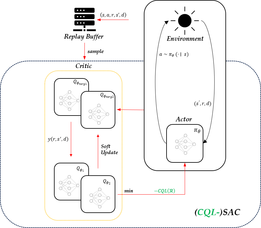
Architecture for SAC and its CQL-modified version is illustrated as follows:

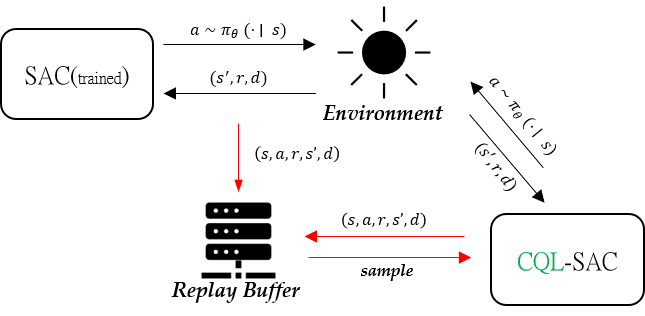
The overall pipeline is visualized below:

pipeline

Pseudocode

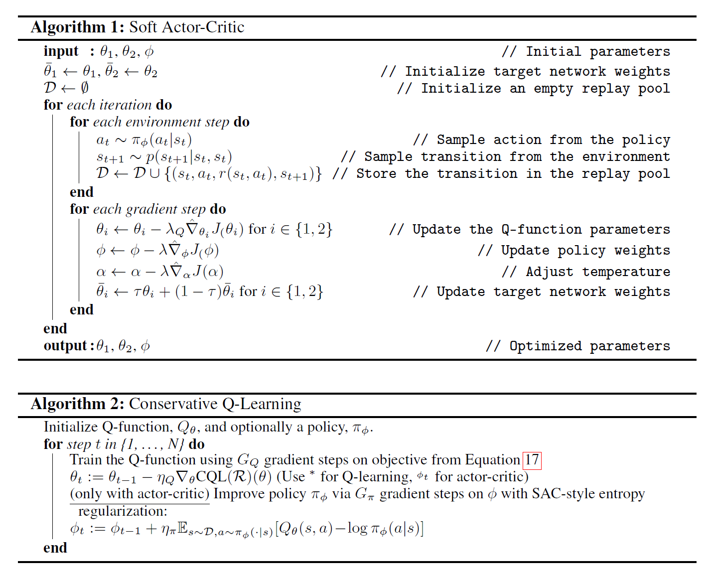
pseudocode

Implementation

For an implementation of the CQL-SAC algorithm, please refer to our Github repo.

References

[1] Spinning Up in Deep Reinforcement Learning, Achiam, Joshua, (2018).

[2] Haarnoja, Tuomas, et al. “Soft actor-critic algorithms and applications.” arXiv preprint arXiv:1812.05905 (2018). [3] Kumar, Aviral, et al. “Conservative q-learning for offline reinforcement learning.” Advances in Neural Information Processing Systems 33 (2020): 1179-1191. [4] Zhang, Shangtong, and Richard S. Sutton. “A deeper look at experience replay.” arXiv preprint arXiv:1712.01275 (2017). [5] Fujimoto, Scott, Herke Hoof, and David Meger. “Addressing function approximation error in actor-critic methods.” International conference on machine learning. PMLR, 2018.

[6] Sergey Levine, Aviral Kumar, George Tucker, and Justin Fu. Offline reinforcement learning: Tutorial, review, and perspectives on open problems. arXiv preprint arXiv:2005.01643, 2020.

[7] Aviral Kumar, Justin Fu, Matthew Soh, George Tucker, and Sergey Levine. Stabilizing off-policy q-learning via bootstrapping error reduction. In Advances in Neural Information Processing Systems, pages 11761–11771, 2019.

[8]Aviral Kumar, Aurick Zhou, George Tucker and Sergey Levine. Conservative q-learning for offline reinforcement learning. In Advances in Neural Information Processing Systems, 2020.